What is Calculus in Machine Learning | April 2021

I. Introduction

A machine learning algorithm (such as classification, clustering or regression) uses a training dataset to determine weight factors that can be applied to unseen data for predictive purposes. Behind every machine learning model is an optimization algorithm that relies heavily on calculus. In this article, we discuss one such optimization algorithm, namely, the Gradient Descent Approximation (GDA) and we’ll show how it can be used to build a simple regression estimator.

II. Optimization Using the Gradient Descent Algorithm

II.1 Derivatives and Gradients

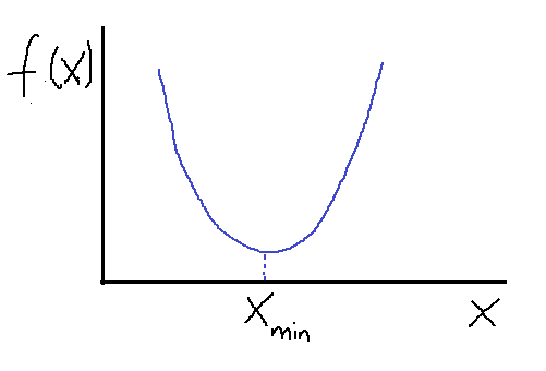
In one-dimension, we can find the maximum and minimum of a function using derivatives. Let us consider a simple quadratic function f(x) as shown below.

Minimum of a simple function using gradient descent algorithm. Image by Benjamin O. Tayo

Suppose we want to find the minimum of the function f(x). Using the gradient descent method with some initial guess, X gets updated according to this equation:

where the constant eta is a small positive constant called the learning rate. Note the following:

• when X_n > X_min, f’(X_n) > 0: this ensures that X_n+1 is less than X_n. Hence we are taking steps in the left direction to get to the minimum.
• when X_n < X_min, f’(X_n) < 0: this ensures that X_n+1 is greater than X_n. Hence we are taking steps in the right direction to get to X_min.

The above observation shows that it doesn’t matter what the initial guess is, the gradient descent algorithm will always find the minimum. How many optimization steps it’s going to take to get to X_min depends on how good the initial guess is. Sometimes if the initial guess or the learning rate is not carefully chosen, the algorithm can completely miss the minimum. This is often referred to as an “overshoot”. Generally, one could ensure convergence by adding a convergence criterion such as:

where epsilon is a small positive number.

In higher dimensions, a function of several variables can be optimized (minimized) using the gradient descent algorithm as well. In this case, we use the gradient to update the vector X:

As in one-dimension, one could ensure convergence by adding a convergence criterion such as:

II.2 Case Study: Building a Simple Regression Estimator

In this subsection, we describe how a simple python estimator can be built to perform linear regression using the gradient descent method. Let’s assume we have a one-dimensional dataset containing a single feature (X) and an outcome (y), and let’s assume there are N observations in the dataset:

A linear model to fit the data is given as:

where w0 and w1 are the weights that the algorithm learns during training.

II.3 Gradient Descent Algorithm

If we assume that the error in the model is independent and normally distributed, then the likelihood function is given as:

To maximize the likelihood function, we minimize the sum of squared errors (SSE) with respect to w0 and w1:

The objective function or our SSE function is often minimized using the gradient descent approximation(GDA) algorithm. In the GDA method, the weights are updated according to the following procedure:

i.e., in the direction opposite to the gradient. Here, eta is a small positive constant referred to as the learning rate. This equation can be written in component form as:

II.4 Python Implementation

import pandas as pd
import numpy as np
import matplotlib.pyplot as plt
class GradientDescent(object):
    """Gradient descent optimizer.
    Parameters
    ------------
    eta : float
        Learning rate (between 0.0 and 1.0)
    n_iter : int
        Passes over the training dataset.
        
    Attributes
    -----------
    w_ : 1d-array
        Weights after fitting.
    errors_ : list
        Error in every epoch.
    """    def __init__(self, eta=0.01, n_iter=10):
        self.eta = eta
        self.n_iter = n_iter
        
    def fit(self, X, y):
        """Fit the data.
        
        Parameters
        ----------
        X : {array-like}, shape = [n_points]
        Independent variable or predictor.
        y : array-like, shape = [n_points]
        Outcome of prediction.
        Returns
        -------
        self : object
        """
        self.w_ = np.zeros(2)
        self.errors_ = []
        
        for i in range(self.n_iter):
            errors = 0
            for j in range(X.shape[0]):
                self.w_[1:] += self.eta*X[j]*(y[j] - self.w_[0] -                     self.w_[1]*X[j])
                self.w_[0] += self.eta*(y[j] - self.w_[0] - self.w_[1]*X[j])
                errors += 0.5*(y[j] - self.w_[0] - self.w_[1]*X[j])**2
            self.errors_.append(errors)
        return self    def predict(self, X):
        """Return predicted y values"""
        return self.w_[0] + self.w_[1]*X

II.5 Application of basic regression model

a) Create dataset

np.random.seed(1)
X=np.linspace(0,1,10)
y = 2*X + 1
y = y + np.random.normal(0,0.05,X.shape[0])

b) Fit and Predict

gda = GradientDescent(eta=0.1, n_iter=100)
gda.fit(X,y)
y_hat=gda.predict(X)

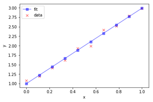
c) Plot Output

plt.figure()
plt.scatter(X,y, marker='x',c='r',alpha=0.5,label='data')
plt.plot(X,y_hat, marker='s',c='b',alpha=0.5,label='fit')
plt.xlabel('x')
plt.ylabel('y')
plt.legend()

Image by Benjamin O. Tayo

d) Calculate R-square value

R_sq = 1-((y_hat - y)**2).sum()/((y-np.mean(y))**2).sum()
R_sq
0.991281901588877

III. Summary and Conclusion

In summary, we have shown how a simple linear regression estimator using the GDA algorithm can be built and implemented in Python. Behind every machine learning model is an optimization algorithm that relies heavily on calculus. If you would like to see how the GDA algorithm is used in a real machine learning classification algorithm, see the following Github repository.

For some Python Code you may follow this GitHub Repository